Here’s a favorite Excel spreadsheet trick:
Say Column D is a list of Dates and you would like to highlight the Row if Today’s date matches. Try the following.
Note: Make sure Column D cells are Formatted as Dates!
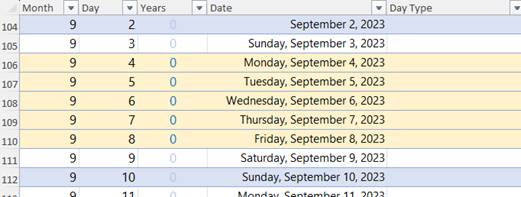
- From the Home ribbon, select the cells you would like the Conditional Formatting to apply.
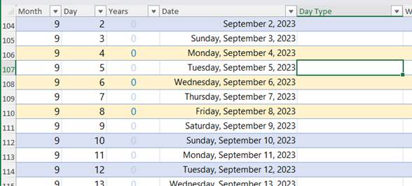
If the desired selection is already an Excel Table, select the entire Excel Table. For example:
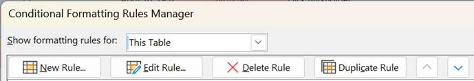
- From the Home ribbon, select Conditional Formatting then Manage Rules…
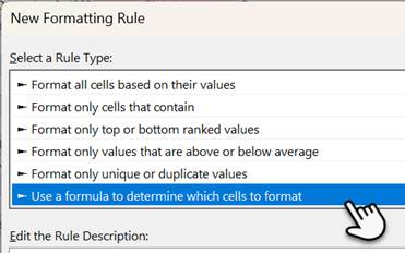
- Select New Rule…
- In New Formatting Rule, select Use a formula to determine which cells to format
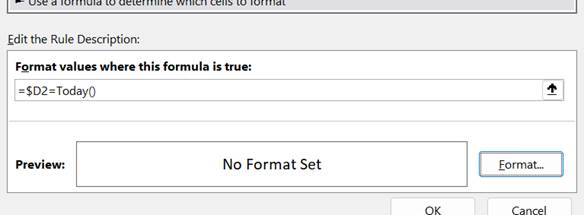
- For Format values where this formulas is true, specify:
=$D2=Today()
Note: In this case, “D” is the column with the Date value. The dollar sign or “$” indicates the column will not change. The row “2” is selected because it is the first row after the header.
- Next select the Format… button.
- Select the Fill tab.
- Choose the Background color you prefer and select OK.
- In the window Conditional Formatting Rules Manager, select OK.
Other Examples:
- If you want to take it up a notch and highlight rows for this week, you use “=WeekNum()” which returns the current Week Number of the year.
=WEEKNUM($D2)=WEEKNUM(TODAY())
Evaluates if the Week Number of the date from Column D equals the Week Number for Today’s Date
- To use conditional formatting for the Next week’s rows, then add One to the Week Number:
=WEEKNUM($D2)=WEEKNUM(TODAY())+1
Or
=WEEKNUM($D2)=(WEEKNUM(TODAY())+1)
Or Add 7 days to Today’s Date for a similar calculation.
=WEEKNUM($D2)=WEEKNUM(TODAY()+DAY(7))
- To use conditional formatting for Previous week’s rows, then subtract One from the Week Number
=WEEKNUM($D2)=WEEKNUM(TODAY())-1
- Maybe you want it highlighted but not on Saturday (1) or Sunday (7), then combine the above using And while evaluating if Column D is greater than Saturday AND less than Sunday
=AND(WEEKNUM($D2)=WEEKNUM(TODAY()-DAY(7)),WEEKDAY($D2)>1,WEEKDAY($D2)<7)
=AND(
WEEKNUM($D2)=WEEKNUM(TODAY()-DAY(7)),
WEEKDAY($D2)>1,
WEEKDAY($D2)<7
)
- Or maybe you want last week highlighted, but only for Monday (2) or Wednesday (4) or Friday (6), then use the AND with the OR
=AND(WEEKNUM($D2)=WEEKNUM(TODAY()-DAY(7)),OR(WEEKDAY($D2)=2,WEEKDAY($D2)=4,WEEKDAY($D2)=6))
=AND(
WEEKNUM($D2)=WEEKNUM(TODAY()-DAY(7)),
OR(
WEEKDAY($D2)=2,
WEEKDAY($D2)=4,
WEEKDAY($D2)=6
)
)